Machine Learning : Naive Bayes

Naive Bayes:

You are working on a classification problem and have generated your set of hypothesis, created features and discussed the importance of variables. Within an hour, stakeholders want to see the first cut of the model.

What will you do? You have hundreds of thousands of data points and quite a few variables in your training data set. In such a situation, if I were in your place, I would have used ‘Naive Bayes‘, which can be extremely fast relative to other classification algorithms. It works on Bayes theorem of probability to predict the class of unknown data sets.

What is Naive Bayes algorithm?

It is a classification technique based on Bayes’ Theorem with an assumption of independence among predictors. In simple terms, a Naive Bayes classifier assumes that the presence of a particular feature in a class is unrelated to the presence of any other feature.

For example, a fruit may be considered to be an apple if it is red, round, and about 3 inches in diameter. Even if these features depend on each other or upon the existence of the other features, all of these properties independently contribute to the probability that this fruit is an apple and that is why it is known as ‘Naive’.

Naive Bayes model is easy to build and particularly useful for very large data sets. Along with simplicity, Naive Bayes is known to outperform even highly sophisticated classification methods.

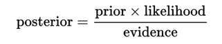
Bayes theorem provides a way of calculating posterior probability P(c|x) from P(c), P(x) and P(x|c). Look at the equation below:

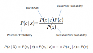
Above,

• P(c|x) is the posterior probability of class (c, target) given predictor (x, attributes).
• P(c) is the prior probability of class.
• P(x|c) is the likelihood which is the probability of predictor given class.
• P(x) is the prior probability of predictor.

 Using the Bayes’ theorem, its possible to build a learner that predicts the probability of the response variable belonging to some class, given a new set of attributes.

How Naive Bayes algorithm works?

Let’s understand it using an example. Below I have a training data set of weather and corresponding target variable ‘Play’ (suggesting possibilities of playing). Now, we need to classify whether players will play or not based on weather condition. Let’s follow the below steps to perform it.

Step 1: Convert the data set into a frequency table

Step 2: Create Likelihood table by finding the probabilities like Overcast probability = 0.29 and probability of playing is 0.64.

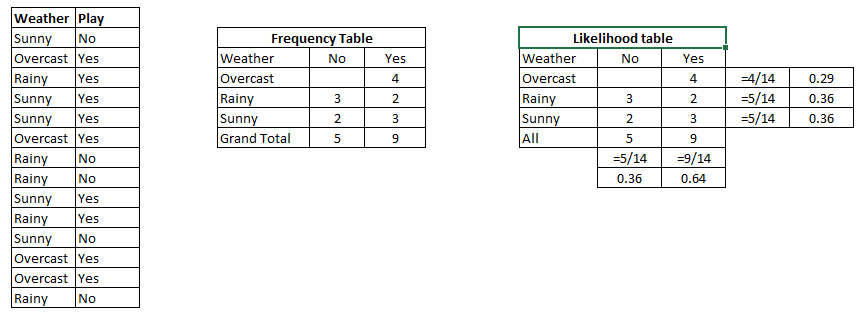
Step 3: Now, use Naive Bayesian equation to calculate the posterior probability for each class. The class with the highest posterior probability is the outcome of prediction.

Problem: Players will play if weather is sunny. Is this statement is correct?

We can solve it using above discussed method of posterior probability.

P(Yes | Sunny) = P( Sunny | Yes) * P(Yes) / P (Sunny)

Here we have P (Sunny |Yes) = 3/9 = 0.33, P(Sunny) = 5/14 = 0.36, P( Yes)= 9/14 = 0.64

Now, P (Yes | Sunny) = 0.33 * 0.64 / 0.36 = 0.60, which has higher probability.

Naive Bayes uses a similar method to predict the probability of different class based on various attributes. This algorithm is mostly used in text classification and with problems having multiple classes.

Let’s take a problem, where the number of attributes is equal to n and the response is a boolean value, i.e. it can be in one of the two classes. Also, the attributes are categorical(2 categories for our case). Now, to train the classifier, we will need to calculate P(B|A), for all the values in the instance and response space. This means, we will need to calculate 2*(2^n -1), parameters for learning this model. This is clearly unrealistic in most practical learning domains. For example, if there are 30 boolean attributes, then we will need to estimate more than 3 billion parameters.

Naive Bayes Algorithm

The complexity of the above Bayesian classifier needs to be reduced, for it to be practical. The naive Bayes algorithm does that by making an assumption of conditional independence over the training dataset. This drastically reduces the complexity of above mentioned problem to just 2n.

The assumption of conditional independence states that, given random variables X, Y and Z, we say X is conditionally independent of Y given Z, if and only if the probability distribution governing X is independent of the value of Y given Z.

In other words, X and Y are conditionally independent given Z if and only if, given knowledge that Z occurs, knowledge of whether X occurs provides no information on the likelihood of Y occurring, and knowledge of whether Y occurs provides no information on the likelihood of X occurring.

This assumption makes the Bayes algorithm, naive.

Maximizing a Posteriori

What we are interested in, is finding the posterior probability or P(Y|X). Now, for multiple values of Y, we will need to calculate this expression for each of them.

Given a new instance Xnew, we need to calculate the probability that Y will take on any given value, given the observed attribute values of Xnew and given the distributions P(Y) and P(X|Y) estimated from the training data.

So, how will we predict the class of the response variable, based on the different values we attain for P(Y|X). We simply take the most probable or maximum of these values. Therefore, this procedure is also known as maximizing a posteriori.

Maximizing Likelihood

If we assume that the response variable is uniformly distributed, that is it is equally likely to get any response, then we can further simplify the algorithm. With this assumption the priori or P(Y) becomes a constant value, which is 1/categories of the response.

As, the priori and evidence are now independent of the response variable, these can be removed from the equation. Therefore, the maximizing the posteriori is reduced to maximizing the likelihood problem.

Feature Distribution

As seen above, we need to estimate the distribution of the response variable from training set or assume uniform distribution. Similarly, to estimate the parameters for a feature’s distribution, one must assume a distribution or generate nonparametric models for the features from the training set. Such assumptions are known as event models. The variations in these assumptions generates different algorithms for different purposes. For continuous distributions, the Gaussian naive Bayes is the algorithm of choice. For discrete features, multinomial and Bernoulli distributions as popular. Detailed discussion of these variations are out of the scope of this article.

Naive Bayes classifiers work really well in complex situations, despite the simplified assumptions and naivety. The advantage of these classifiers is that they require small number of training data for estimating the parameters necessary for classification. This is the algorithm of choice for text categorization. This is the basic idea behind naive Bayes classifiers, that you need to start experimenting with the algorithm.

 

What are the Pros and Cons of Naive Bayes?

Pros:

• It is easy and fast to predict class of test data set. It also perform well in multi class prediction
• When assumption of independence holds, a Naive Bayes classifier performs better compare to other models like logistic regression and you need less training data.
• It perform well in case of categorical input variables compared to numerical variable(s). For numerical variable, normal distribution is assumed (bell curve, which is a strong assumption).

Cons:

• If categorical variable has a category (in test data set), which was not observed in training data set, then model will assign a 0 (zero) probability and will be unable to make a prediction. This is often known as “Zero Frequency”. To solve this, we can use the smoothing technique. One of the simplest smoothing techniques is called Laplace estimation.
• On the other side naive Bayes is also known as a bad estimator, so the probability outputs from predict_proba are not to be taken too seriously.
• Another limitation of Naive Bayes is the assumption of independent predictors. In real life, it is almost impossible that we get a set of predictors which are completely independent.

4 Applications of Naive Bayes Algorithms

• Real time Prediction: Naive Bayes is an eager learning classifier and it is sure fast. Thus, it could be used for making predictions in real time.
• Multi class Prediction: This algorithm is also well known for multi class prediction feature. Here we can predict the probability of multiple classes of target variable.
• Text classification/ Spam Filtering/ Sentiment Analysis: Naive Bayes classifiers mostly used in text classification (due to better result in multi class problems and independence rule) have higher success rate as compared to other algorithms. As a result, it is widely used in Spam filtering (identify spam e-mail) and Sentiment Analysis (in social media analysis, to identify positive and negative customer sentiments)
• Recommendation System: Naive Bayes Classifier and Collaborative Filtering together builds a Recommendation System that uses machine learning and data mining techniques to filter unseen information and predict whether a user would like a given resource or not

 

How to build a basic model using Naive Bayes in Python?

Again, scikit learn (python library) will help here to build a Naive Bayes model in Python. There are three types of Naive Bayes model under the scikit-learn library:

• Gaussian: It is used in classification and it assumes that features follow a normal distribution.

• Multinomial: It is used for discrete counts. For example, let’s say,  we have a text classification problem. Here we can consider Bernoulli trials which is one step further and instead of “word occurring in the document”, we have “count how often word occurs in the document”, you can think of it as “number of times outcome number x_i is observed over the n trials”.

• Bernoulli: The binomial model is useful if your feature vectors are binary (i.e. zeros and ones). One application would be text classification with ‘bag of words’ model where the 1s & 0s are “word occurs in the document” and “word does not occur in the document” respectively.

Tips to improve the power of Naive Bayes Model

Here are some tips for improving power of Naive Bayes Model:

• If continuous features do not have normal distribution, we should use transformation or different methods to convert it in normal distribution.
• If test data set has zero frequency issue, apply smoothing techniques “Laplace Correction” to predict the class of test data set.
• Remove correlated features, as the highly correlated features are voted twice in the model and it can lead to over inflating importance.
• Naive Bayes classifiers has limited options for parameter tuning like alpha=1 for smoothing, fit_prior=[True|False] to learn class prior probabilities or not and some other options (look at detail here). I would recommend to focus on your  pre-processing of data and the feature selection.
• You might think to apply some classifier combination technique like ensembling, bagging and boosting but these methods would not help. Actually, “ensembling, boosting, bagging” won’t help since their purpose is to reduce variance. Naive Bayes has no variance to minimize.