Machine Learning:SVM

 What is Support Vector Machine?

“Support Vector Machine” (SVM) is a supervised machine learning algorithm which can be used for both classification or regression challenges. However,  it is mostly used in classification problems. In the SVM algorithm, we plot each data item as a point in n-dimensional space (where n is number of features you have) with the value of each feature being the value of a particular coordinate. Then, we perform classification by finding the hyper-plane that differentiates the two classes very well (look at the below snapshot).

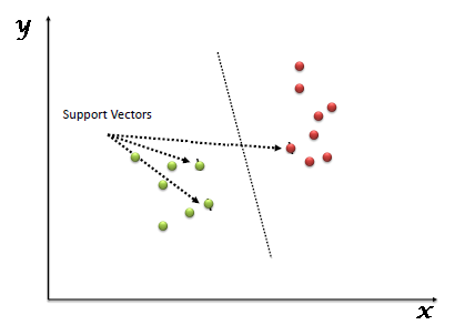
Support Vectors are simply the co-ordinates of individual observation. The SVM classifier is a frontier which best segregates the two classes (hyper-plane/ line).

How does it work?

Above, we got accustomed to the process of segregating the two classes with a hyper-plane. Now the burning question is “How can we identify the right hyper-plane?”. Don’t worry, it’s not as hard as you think!

Let’s understand:

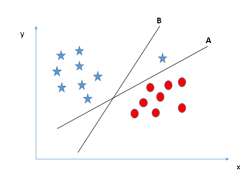
• Identify the right hyper-plane (Scenario-1): Here, we have three hyper-planes (A, B and C). Now, identify the right hyper-plane to classify star and circle.

 

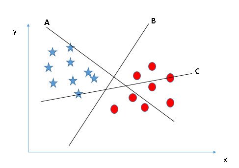
• You need to remember a thumb rule to identify the right hyper-plane: “Select the hyper-plane which segregates the two classes better”. In this scenario, hyper-plane “B” has excellently performed this job.
• Identify the right hyper-plane (Scenario-2): Here, we have three hyper-planes (A, B and C) and all are segregating the classes well. Now, How can we identify the right hyper-plane?

Here, maximizing the distances between nearest data point (either class) and hyper-plane will help us to decide the right hyper-plane. This distance is called as Margin. Let’s look at the below snapshot:

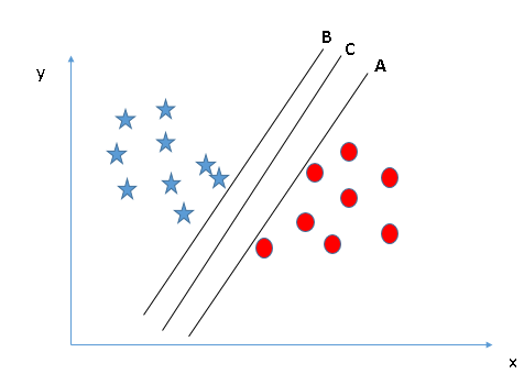
• Above, you can see that the margin for hyper-plane C is high as compared to both A and B. Hence, we name the right hyper-plane as C. Another lightning reason for selecting the hyper-plane with higher margin is robustness. If we select a hyper-plane having low margin then there is high chance of miss-classification.

Identify the right hyper-plane (Scenario-3):Hint: Use the rules as discussed in previous section to identify the right hyper-plane

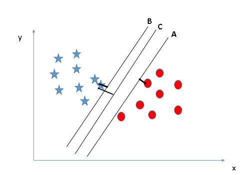
Some of you may have selected the hyper-plane B as it has higher margin compared to A. But, here is the catch, SVM selects the hyper-plane which classifies the classes accurately prior to maximizing margin. Here, hyper-plane B has a classification error and A has classified all correctly. Therefore, the right hyper-plane is A.

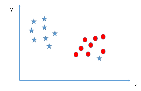
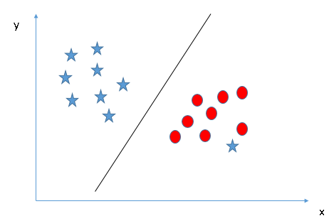
• Can we classify two classes (Scenario-4)?: Below, I am unable to segregate the two classes using a straight line, as one of the stars lies in the territory of other(circle) class as an outlier. 

As I have already mentioned, one star at other end is like an outlier for star class. The SVM algorithm has a feature to ignore outliers and find the hyper-plane that has the maximum margin. Hence, we can say, SVM classification is robust to outliers.

Find the hyper-plane to segregate to classes (Scenario-5): In the scenario below, we can’t have linear hyper-plane between the two classes, so how does SVM classify these two classes? Till now, we have only looked at the linear hyper-plane.

SVM can solve this problem. Easily! It solves this problem by introducing additional feature. Here, we will add a new feature z=x^2+y^2. Now, let’s plot the data points on axis x and z:

In above plot, points to consider are:

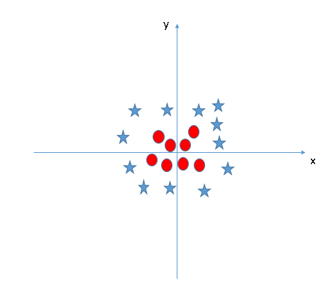
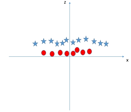
• All values for z would be positive always because z is the squared sum of both x and y
• In the original plot, red circles appear close to the origin of x and y axes, leading to lower value of z and star relatively away from the origin result to higher value of z.

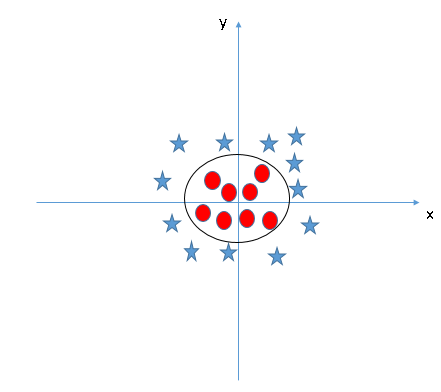
In the SVM classifier, it is easy to have a linear hyper-plane between these two classes. But, another burning question which arises is, should we need to add this feature manually to have a hyper-plane. No, the SVM  algorithm has a technique called the kernel trick. The SVM kernel is a function that takes low dimensional input space and transforms it to a higher dimensional space i.e. it converts not separable problem to separable problem. It is mostly useful in non-linear separation problem. Simply put, it does some extremely complex data transformations, then finds out the process to separate the data based on the labels or outputs you’ve defined.

When we look at the hyper-plane in original input space it looks like a circle:

Large Margin Intuition

 In SVM, we take the output of the linear function and if that output is greater than 1, we identify it with one class and if the output is -1, we identify is with another class. Since the threshold values are changed to 1 and -1 in SVM, we obtain this reinforcement range of values([-1,1]) which acts as margin.

Cost Function and Gradient Updates

In the SVM algorithm, we are looking to maximize the margin between the data points and the hyperplane. The loss function that helps maximize the margin is hinge loss.

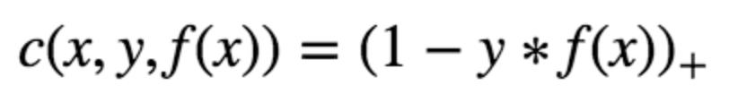
Hinge loss function (function on left can be represented as a function on the right)

The cost is 0 if the predicted value and the actual value are of the same sign. If they are not, we then calculate the loss value. We also add a regularization parameter the cost function. The objective of the regularization parameter is to balance the margin maximization and loss. After adding the regularization parameter, the cost functions looks as below.

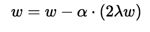
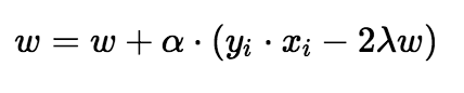
Now that we have the loss function, we take partial derivatives with respect to the weights to find the gradients. Using the gradients, we can update our weights.

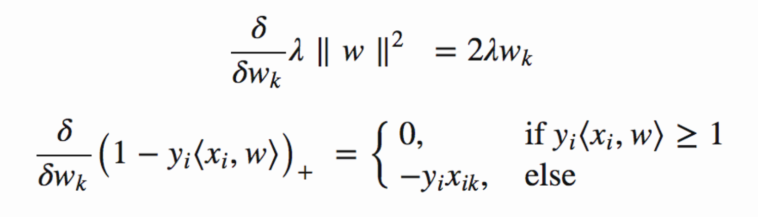
When there is no misclassification, i.e our model correctly predicts the class of our data point, we only have to update the gradient from the regularization parameter.

When there is a misclassification, i.e our model make a mistake on the prediction of the class of our data point, we include the loss along with the regularization parameter to perform gradient update.

SVM is a Linear Model and Kernel SSM is a Non-linear SVM