Covariance & Correleation Matrix Pearson Correlation

In probability covariance is the measure of the joint probability for two random variables. It describes how the two variables change together 

It is denoted as the function cov(X,Y) Where X and Y are the two random variables being considered 

cov(X,Y)

Covariance is calculated as the expected value or average of the product of the differences of each variable from theor expectedvalues ,Where E[X] is the expected value for X and E(Y) is the expected value of y.

in simple terms 

cov(X,Y)=E[ ( X - E[X] ) . ( Y - E[Y] ) ]

for n values 

cov(X,Y)=sum(E[ ( X - E[X] ) . ( Y - E[Y] ) ]) * 1/n

or,

cov(X,Y)=sum([ ( X - X^ ) . ( Y - Y^ ) ]) * 1/n 

sum is upto n

The sign indicates that whether two variables increase together or decrease together.

+ve sign means value are increasing and -ve means value are decreasing 

A variance value of zero are completely indicated that both variables are independent

in numpy we use conv()  to find covariance

Note. It doesn't show how much negativity and positivity it brings so for this we calculate correlation

PEARSON CORRELATION COEFFICIENT.

It always range between -1<corr<1

corr=cov(x,y)/standard_deviation(X)*standard_deviation(Y)

X increasing,Y increasing   then corr=1

X decreasing,Y increasing   then corr=-1

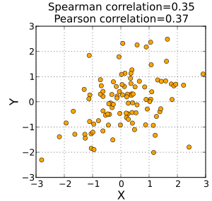
when I have a scatter plot then my covariance is 0 because in scater plot when my X is increasing and y is decreasing and vice versa 

When some of the points fitted the line and X is decreasing and Y is Increasing then My corr is from -1 <corr<0

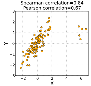
When some of the points fittedthe line and X is increasing and Y is increasing then my corr is from 0 to 1 

SPEARMAN'S RANK CORRELATION:

In Spearman correlation we use rank instead of x we use their ranks to find out the correlation between them

This is the formula we use to calculate the spearman correlation

1. Sort the data by the first column (${\displaystyle X_{i}}$). Create a new column ${\displaystyle x_{i}}$ and assign it the ranked values 1, 2, 3, ..., n.
2. Next, sort the data by the second column (${\displaystyle Y_{i}}$). Create a fourth column ${\displaystyle y_{i}}$ and similarly assign it the ranked values 1, 2, 3, ..., n.
3. Create a fifth column ${\displaystyle d_{i}}$ to hold the differences between the two rank columns (${\displaystyle x_{i}}$ and ${\displaystyle y_{i}}$).
4. Create one final column ${\displaystyle d_{i}^{2}}$ to hold the value of column ${\displaystyle d_{i}}$ squared.

IQ, ${\displaystyle X_{i}}$	Hours of TV per week, ${\displaystyle Y_{i}}$
106	7
100	27
86	2
101	50
99	28
103	29
97	20
113	12
112	6
110	17

IQ, ${\displaystyle X_{i}}$	Hours of TV per week, ${\displaystyle Y_{i}}$	rank ${\displaystyle x_{i}}$	rank ${\displaystyle y_{i}}$	${\displaystyle d_{i}}$	${\displaystyle d_{i}^{2}}$
86	2	1	1	0	0
97	20	2	6	−4	16
99	28	3	8	−5	25
100	27	4	7	−3	9
101	50	5	10	−5	25
103	29	6	9	−3	9
106	7	7	3	4	16
110	17	8	5	3	9
112	6	9	2	7	49
113	12	10	4	6	36

With ${\displaystyle d_{i}^{2}}$ found, add them to find ${\displaystyle \sum d_{i}^{2}=194}$. The value of n is 10. These values can now be substituted back into the equation

${\displaystyle \rho =1-{\frac {6\sum d_{i}^{2}}{n(n^{2}-1)}}}$

to give

${\displaystyle \rho =1-{\frac {6\times 194}{10(10^{2}-1)}},}$

which evaluates to ρ = −29/165 = −0.175757575... with a p-value = 0.627188 (using the t-distribution).

That the value is close to zero shows that the correlation between IQ and hours spent watching TV is very low, although the negative value suggests that the longer the time spent watching television the lower the IQ.

Little Standard Error show less collinearity between variables

If their is high collinearity between two variables ad if we want to remove the collinearity between them then we just drop them by seeing the P value of any one of them whichever variable have high P value then we drop that variable